Economics
Here we provide examples of solutions and price/time deadlines of students' work that we have solved in the past. If while looking at these examples you find yourself wishing someone could have done that for you? then go ahead and place an order now. We can't wait to help you make your college experience stress free and fun! Place an Order
Subject: Microeconomics. Type: Homework. Due date: 1 day. Price: $7
1.For each of the following scenarios, demonstrate the effect on price and quantity using a supply and demand diagram.
-
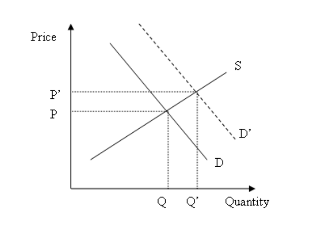
A sudden snowstorm hits the West Coast resulting in a foot of snow. Demonstrate the effect in the winter jacket market in California.
Solution:
The sudden snowstorm shifts the demand curve to the right (or up) from D to D’ since people will be in higher demand of winter jackets. This results in an increase in equilibrium price and quantity (as indicated by P’ and Q’ respectively)

-
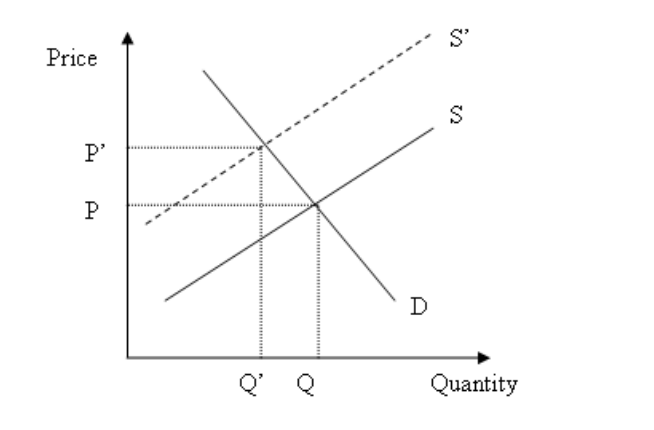
Workers in Canada producing heavy winter jackets are on strike. Demonstrate the effect on the West Coast jacket market.
Solution:
Since the Canadian workers are on strike, there will be fewer jackets produced. Thus, the supply curve will shift left (or up) from S to S’. This results in a decrease in quantity and an increase in price (as indicted by Q’ and P’ respectively).

-
Suppose now the government imposes a tax on winter hats, which the producer pays. Demonstrate the effect on the hat market.
Solution:
Since the government imposes a tax on the producer, the supply curve will shift left (or up) by the amount of the tax from S to S’. This results in a decrease in quantity and an increase in price (as indicated by Q’ and P’ respectively).

2. Suppose you are given the following production function:
Y = KαN1-α where α = 1/4
-
Is this production function characterized by constant returns to scale? Explain.
Solution:
To check whether a function has constant returns to scale:
F(aK, aN) = aF(K, N)In this example:
(aK)α (aN)1-α = aα a1-α Kα N1- α = aKα N1-αThus, this production function is characterized by constant returns to scale.
-
Are there decreasing returns to capital?
Solution:
To check whether a function has decreasing returns to capital, we take the derivate with respect to capital (K). We can also note that the exponent on the variable for capital (K) is less than 1.
Thus, there is decreasing returns to capital.
-
Are there decreasing returns to labor?
Solution:
To check whether a function has decreasing returns to labor, we take the derivate with respect to labor (N). We can also note that the exponent on the variable for labor (N) is less than 1.
Thus, there is decreasing returns to labor.
-
Transform the production function into a relation between output per worker and capital per worker.
Solution:
Output per worker is Y/N therefore we divide both sides by N
$\frac{Y}{N} = \left ( \frac{K}{N} \right )^{\alpha }$ -
For a given saving rate, s, and depreciation rate, δ, given an expression for capital per worker in the steady state.
Solution:
In the steady state:
K* = (1 - δ)K* + sY*We can divide this equation by N:
$\frac{K^{*}}{N} = (1 - \delta )\frac{K^{*}}{N} + S\frac{Y^{*}}{N}$Let’s rename $\frac{K^{*}}{N}$ as k* and use the relation from part d:
k* = (1 - δ)k* + sk*α -
We can now solve for k*:
${k^{*}} = \left ( \frac{s}{\delta } \right )^{\frac{1}{1-\alpha}} = \left ( \frac{s}{\delta } \right )^{\frac{1}{3}}$ -
Give an expression for output per worker in the steady state.
Solution:
${y^{*}} = {k^{*}} = \left ( \frac{s}{\delta } \right )^{\frac{1}{3}}$ -
Solve for the steady state level of output per worker when s = 0.2 and = 0.025
Solution:
-
Plugging in the values given to the equation from part f:
${y^{*}} = \left ( \frac{0.2}{0.025 } \right )^{\frac{1}{3}} = 2$ -
Now suppose the savings rate is reduced to 0.1, while the depreciation rate remains the same. What is the new steady-state output per worker?
Solution:
${y^{*}} = \left ( \frac{0.1}{0.025 } \right )^{\frac{1}{3}} = \sqrt[3]{4}$
3. Suppose you are given the following game with payoffs as indicated in each cell:
| Player 1, Player 2 | Collude | Diverge |
| Collude | (2, 1) | (0, 0) |
| Diverge | (0, 3) | (3, 3) |
-
Find the Nash Equilibrium
Solution:
If player 1 colludes, then player 2 will prefer to collude.
If player 1 diverges, then player 2 is indifferent.
If player 2 colludes, then player 1 will prefer to collude.
If player 2 diverges, then player 1 will prefer to diverge.
Thus, the Nash Equilibrium is (Collude, Collude) and (Diverge, Diverge)
-
Find the mixed strategy equilibrium
Solution:
To find the mixed strategy equilibrium each player must be indifferent between playing each of his or her strategies.
Suppose the probability with which player 1 plays Collude is p and the probability with which player 2 plays Collude is q.
Payoff Player 1 playing collude = Payoff Player 1 playing diverge
2p + 0(1 - p) = 0p + 3(1 - p)
p = 3/5Payoff Player 2 playing collude = Payoff Player 2 playing diverge
1q + 2(1 - q) = 0q + 3(1 - q)
q = 1/2 -
Are all Nash Equilibria Pareto efficient? If not, give a contradictory example.
Solution:
Not all Nash Equilibria are Pareto efficient. A contradictory example would be the prisoner’s dilemma where both players would be strictly better off if they cooperated, but in the Nash equilibrium they both choose to deviate.
Player 1, Player 2 Cooperate Deviate Cooperate (-1, -1) (-3, 0) Deviate (0, -3) (-2, -2) Here we see that the Nash equilibrium is (Deviate, Deviate), but both players’ payoff would be higher if they choose to cooperate.
-
Is there a dominant strategy for either player?
Solution:
In this game we do not see a dominant strategy for either player. If there was a dominant strategy for either player, then that player would choose to play that strategy regardless of what the other player plays.
